Decision boundary plot

0) Load the required R packages

library('geomorph') #  geometric morphometric functions
## Loading required package: RRPP
## Loading required package: rgl
## Loading required package: Matrix
library('caret') # to carry out the lda
## Loading required package: lattice
## Loading required package: ggplot2

1) Import the Data

First we load the data which in this example consists of 30 3D coordinates that were collected on the surface of the tali (i.e., astragali) of both extinct and extant fossil New World monkeys

# this data corresponds to the talar shape data analysed in the paper
load('Talar_shape.RData')

2) Geometric morphometric analysis and PCA

Now we carried out a Procrustes superimposition to remove the differences due to scale, translation and rotation, leaving only variables directly related to shape. Then, these shape variables were used to carry out a principal component analysis (PCA) to visualize morphological affinities.

names <-tmp[,1] # define names
coords <-(arrayspecs(tmp[,7:ncol(tmp)], 30, 3)) # Convert landmark data matrix into array
dimnames(coords)[[3]] <-names
proc<-gpagen(coords) # Procrustes superimposition 
z<-two.d.array(proc$coords) #arrange coordinate as a 2D array 

There was no need to perform any additional pre-processing procedure prior to the application of the LDA, given that the original raw coordinates were subjected to a Procrustes superimposition, which centered each configuration of landmarks at the origin, scaled them to unit centroid size and rotated them to optimal alignment on the average shape. In addition, a PCA was carried out using these shape coordinates to avoid any possible collinearity.

# compute PCA
PCA_morpho = prcomp(z, scale=F)
# plot PCA
PCs <- data.frame(PCA_morpho$x, tmp[,1:7])
# A basic scatterplot with color depending on Species
p1<- ggplot(PCs, aes(x=PC1, y=PC2, color=Locomotion)) + geom_point(size=6)
p1+scale_color_manual(values=c("#DE7862",  "#E75B64", "#278B9A", "#5A6F80"))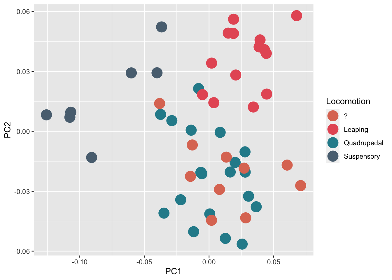

3) Linear Discriminant Analysis

The LDA was computed using the first two PCs obtained from the above PCA (this was done for simplicity in this example). The performance of the classification models was quantified using the confusion matrix from which the overall classification accuracy (i.e. error rate) was computed, as well as by computing Cohen’s Kappa coefficient. To assess the performance of the models, the complete dataset was resampled using a ‘leave-group-out’ cross-validation. The obatained discriminant equation was then used to classify the fossil sample into locomotor categories.

#prepare dataset for caret
# here only a linear discriminant analysis (LDA) was modeled for simplicity
locomotion<-tmp[1:40,]$Locomotion
train<-data.frame(PCA_morpho$x[1:40,1:2],locomotion) #Join the above data
train$locomotion<-factor(train$locomotion)
test<-as.data.frame(PCA_morpho$x[41:50,1:2]) # this is the fossil data
# define control cross-validation and metric to be used for performance
control <- trainControl(method="LGOCV", number= 200, classProbs=T) #‘leave-group-out’ cross-validation
metric <- "Accuracy" 

#LDA
set.seed(2666) # set seed to ensure reproducibility (this number was chosen as an homage to Roberto Bolaño's homonymous novel)
fit.lda <- train(locomotion~., data=train, method="lda", metric=metric, trControl=control)
fit.lda
## Linear Discriminant Analysis 
## 
## 40 samples
##  2 predictor
##  3 classes: 'Leaping', 'Quadrupedal', 'Suspensory' 
## 
## No pre-processing
## Resampling: Repeated Train/Test Splits Estimated (200 reps, 75%) 
## Summary of sample sizes: 32, 32, 32, 32, 32, 32, ... 
## Resampling results:
## 
##   Accuracy  Kappa    
##   0.9375    0.8967895

# classify the fossil specimens
# obtain posterior probabilities and classes
predictions<-predict(fit.lda, test, type="prob") 
predictions
##                                   Leaping Quadrupedal   Suspensory
## Aotus_dindensis              0.0035766196   0.9964105 1.285367e-05
## Carlocebus_carmenensis       0.0399511767   0.9600089 3.993250e-05
## Cebupithecia_sarmientoi      0.0008409704   0.9991589 1.156270e-07
## Dolichocebus_gaimanensis     0.0047781457   0.9944489 7.729921e-04
## Madre_de_Dios                0.0824187790   0.9175812 2.291309e-08
## Neosaimiri_fieldsi           0.0003345112   0.9996606 4.924070e-06
## Paralouatta_marianae         0.1219512426   0.2795519 5.984968e-01
## Proteropithecia_neuquenensis 0.0272565400   0.9727407 2.724982e-06
## Rio_Cisnes                   0.0273239195   0.9726761 1.495259e-09
## Soriacebus_ameghinorum       0.0444373587   0.9515617 4.000948e-03
classes<-predict(fit.lda, test)
# join predicted class to test/fossil dataset
test<-data.frame(test,locomotion=classes)

4) Decision boundary plot

Using the above results we can now generate our decision boundary plot

# create prediction grid
# please note that if we were plotting more than  two variables the remaining variables will need to be constrained at 0
# use the 'by' argument to define cell size in the grid
lgrid <- expand.grid(PC1=seq(min(train$PC1), max(train$PC1), by=0.005), 
                     PC2=seq(min(train$PC1), max(train$PC1), by=0.005))


# compute predicted grid
ldaPredGrid <- predict(fit.lda, newdata=lgrid)
ldaPredGrid <- as.numeric(ldaPredGrid)
#
# compute grid probabilities
ldaPredGrid_prob <-predict(fit.lda, newdata=lgrid, type = 'prob')

# loop to obtain the highest probability of belonging to a class/category for each one of the grid cells
prob<-NULL
for (i in 1:dim(ldaPredGrid_prob)[1]){
  prob[i]<-as.numeric(max(ldaPredGrid_prob[i,]))
}
  
# colors for the locomotor groups
bg.cols<-c("#E75B64", "#278B9A", "#5A6F80")

#plot decision boundary
p<-ggplot(data=lgrid, mapping = aes(x=PC1, y=PC2))+
  geom_raster(data = lgrid, mapping = aes(fill=ldaPredGrid), alpha=prob)+
  scale_fill_gradientn(colours=bg.cols,breaks = c(1, 2, 3),labels = c("leaper", "quadruped", "suspensory"))+
  guides(fill = guide_legend(title="locomotor prediction"))


p<-p+geom_point(data = test, aes(x=PC1, y=PC2, shape=locomotion), show.legend = F,colour = '#DE7862', size=5) 

p+geom_point(data = train, aes(x=PC1, y=PC2, shape=locomotion),colour = 'black', size=5) +
   theme(#legend.title = element_text(size=14,color = c("black")), 
         #legend.text = element_text(size=12)
     )+
    labs(title = "Decision boundary plot", caption="Source: thomaspuschel.com")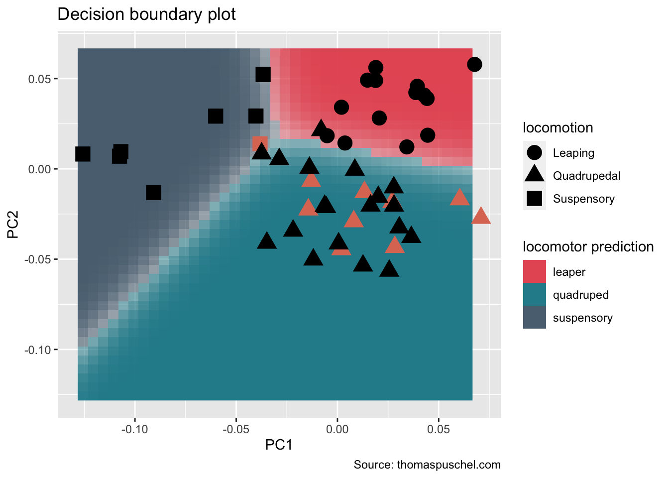 

As you can see most fossils (i.e., salmon-colored shapes) were classified as ‘quadrupeds’, excepting one fossil that was classified as a ‘suspensory’. This latter specimen is quite interesting as it probably represents a locomotor mode unknown for New World monkeys; you can find out more about it here.